#

SOMD MD tutorial ####Step Two: Equilibration

Now we will use the minimised Lysozyme in water file generated in the previous step and equilibrate it. The minimisation was done to make sure that the generated starting structure does not have any overlapping atoms and when running some steps of dynamics will actually make sure the simulation does not ‘explode’, i.e. the forces between atoms are not too large.

The NVT ensemble (constant number of particles, constant volume and constant temperature) simulation is used to make sure that the water molecules orient themselves properly around the protein. For this reason we will restrain the positions of the protein and only let the water relax around the fixed protein. The position restraint means that the protein will stay in the configuration of the X-ray structure, this avoids adding any unnecessary structural changes in the protein before starting the production run of the simulation.

The second part of the equilibration is to simulated an isothermal-isobaric ensemble (NPT) such that the system will relax to the correct volume. Again the position of the protein atoms will still be restraint.

###NVT equilibration

Let’s start by copying the files from the minimisation into a new directory in the top tutorial directory you set up during step one.

cd /path/to/tutorial/
mkdir Equib
cd Equib
mkdir nvt
mkdir npt
cd nvt
cp ../../FESetup/_proteins/1AKI/solvated.parm7 ../1AKI.parm7
cp ../../FESetup/_proteins/1AKI/min00001.rst7 1AKI.rst7

The topology file 1AKI.parm7 can be used for both the NVT and NPT part of the equilibration, which is the reason for not copying into these directories, but instead leave it in the top directory for the equilibration. Simply copy the nvt.cfg file into the nvt directory. We can now run our NVT equilibration by simply running.

somd -C nvt.cfg

This will run the equilibration and a bunch of output will be printed to screen.

If everything ran successfully a few more files will have been generated.

traj000000001.dcd
SYSTEM.s3
sim_restart.s3
moves.dat

The .dcd file is the trajectory file that can, for example, be opened using VMD. *.s3 files are Sire files, holding information of the system and allowing a restart. If a restart file is present, then the simulation will restart from that point, however generating a new trajectory.

Let’s have a bit more detailed look at the configuration file and explain a couple of things in it.

# Length of simulation and platform
nmoves = 500
ncycles = 10        # 500 moves x 10    cycles x 1 fs = 5 ps
platform = CUDA 

Sire works in cycles rather than just a straight forward number of steps. This means that the total number of steps that are meant to be carried out are nmoves*ncycles. The platform flag allows to set different available OpenMM platforms. OpenMM supports four platforms: CUDA, OpenCL, CPU, and Reference. Depending on the computer you are running SOMD on, not all of them will be supported. Please check the OpenMM documentation to find out which ones your computer supports. A safe, but slow bet is the CPU platform. Next we can look at some of the simulation parameters.

# MD integration parameters
timestep = 1 * femtosecond
# Temperature/Pressure control
andersen = True
temperature = 298.15 * kelvin
andersen frequency = 10
barostat = False 

timestep sets the integration timestep, andersen = True turns on the thermostat. Note that units have to be set explicitly. Restraints and output saving is done in the following way:

#restraints on the solute, i.e. protein
use_restraints = True
save coordinates = True

when use_restraint = True then this will only be applied to solute atoms.

###NPT Equilibration First we will have to extract the coordinates of the last frame of the NVT trajectory. Below is an example of how this can be done, but there are many other options too.

1. Install MDtraj via conda if you haven’t done so already:

   ~/sire.app/bin/conda install mdtraj
   Proceed ([y]/n)? y

2. Start ipython from sire and extract the last frame of your nvt trajectory.

   cd ../npt
   ~/sire.app/bin/ipython 
   import mdtraj as md
   t = md.load('../nvt/traj000000001.dcd', top='../1AKI.parm7') #loading trajectory and topology. 
   t[-1].save('nvt.rst7') #saving last frame
   exit

Now we can run the NPT equilibration using the npt.cfg file. This is simply done in the same way as before.

somd -C npt.cfg

After a successful run you should again see the following additional files in your current working directory. If everything ran successfully a few more files will have been generated.

traj000000001.dcd
SYSTEM.s3
sim_restart.s3
moves.dat

If you look at the npt.cfg file you will notice that there are two obvious changes. The coordinate file is now set to the file we just created with the nvt equilibration and the barostat was set to True and a barostat frequency is set too, though the default option should be ok:

crdfile = nvt.rst7
[...]
barostat = True
barostat frequency = 25

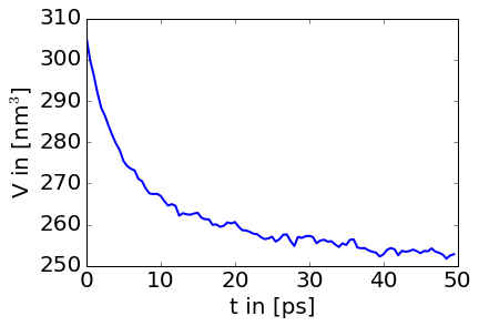
Before we move on to the production run, lets have a quick look at how the volume decreases over the NPT equilibration trajectory. The following few lines of python will let you plot a volume over time plot. (You may have to install matplotlib first ~sire.app/bin/conda install matplotlib and then start ipython that comes with sire as per usual with ~/sire.app/bin/ipython).

import matplotlib.pylab as plt
matplotlib.rcParams.update({'font.size': 20})
import mdtraj as md
t = md.load('traj000000001.dcd', top='../1AKI.parm7')
plt.plot(t.time*0.5, t.unitcell_volumes, linewidth=2)
plt.xlabel(t in [ps]')
plt.ylabel(r'V in [nm$^3$]')

The box volume will fluctuate over time and eventually converge to an equilibrated value. The code above should result in a plot that looks like this:

###Equilibration cheat In fact there is a shortcut to doing an equilibration, which is simply setting the equilibration=True flag in the somd config file. This will run and NVT and NPT equilibration similar to what is described above. Sometimes it is however necessary to manually equilibrate the system you are working with, which makes it worth while understanding the concept and steps required for the equilibration.